Advantages of the multidimensional database model and cube modeling
Discover the advantages of the multidimensional database model and find out how data warehouse cube modeling, data restricting and data slicing work. Learn the role meta-data plays and get a definition of functional dependency.
 |
|
This book excerpt from Data Warehouse Design: Modern Principles and Methodologies discusses the importance and advantages of multidimensional databases, explains how data warehouse cube modeling works and discusses data restricting and data slicing . The excerpt also covers the roles internal and external meta-data play in data warehousing, reviews data aggregation and defines functional dependency.
Table of contents:
![]() An introduction to data warehousing
An introduction to data warehousing
![]() Data warehouse architectures, concepts and phases
Data warehouse architectures, concepts and phases
![]() The advantages of multidimensional databases and cube modeling
The advantages of multidimensional databases and cube modeling
![]() Best practices for data warehouse access and reports
Best practices for data warehouse access and reports
![]() Similarities and differences between ROLAP, MOLAP and HOLAP
Similarities and differences between ROLAP, MOLAP and HOLAP

1.5 Multidimensional Model
The data warehouse layer is a vitally important part of this book. Here, we introduce a data warehouse key word: multidimensional. You need to become familiar with the concepts and terminology used here to understand the information presented throughout this book, particularly information regarding conceptual and logical modeling and designing.
|
||||
Over the last few years, multidimensional databases have generated much research and market interest because they are fundamental for many decision-making support applications, such as data warehouse systems. The reason why the multidimensional model is used as a paradigm of data warehouse data representation is fundamentally connected to its ease of use and intuitiveness even for IT newbies. The multidimensional model's success is also linked to the widespread use of productivity tools, such as spreadsheets, that adopt the multidimensional model as a visualization paradigm.
Perhaps the best starting point to approach the multidimensional model effectively is a definition of the types of queries for which this model is best suited. Section 1.7 offers more details on typical decision-making queries such as those listed here (Jarke et al., 2000):
- "What is the total amount of receipts recorded last year per state and per product category?"
- "What is the relationship between the trend of PC manufacturers' shares and quarter gains over the last five years?"
- "Which orders maximize receipts?"
- "Which one of two new treatments will result in a decrease in the average period of admission?"
- "What is the relationship between profit gained by the shipments consisting of less than 10 items and the profit gained by the shipments of more than 10 items?"
It is clear that using traditional languages, such as SQL, to express these types of queries can be a very difficult task for inexperienced users. It is also clear that running these types of queries against operational databases would result in an unacceptably long response time.
The multidimensional model begins with the observation that the factors affecting decision-making processes are enterprise-specific facts, such as sales, shipments, hospital admissions, surgeries, and so on. Instances of a fact correspond to events that occurred. For example, every single sale or shipment carried out is an event. Each fact is described by the values of a set of relevant measures that provide a quantitative description of events. For example, sales receipts, amounts shipped, hospital admission costs, and surgery time are measures.
Obviously, a huge number of events occur in typical enterprises—too many to analyze one by one. Imagine placing them all into an n-dimensional space to help us quickly select and sort them out. The n-dimensional space axes are called analysis dimensions, and they define different perspectives to single out events. For example, the sales in a store chain can be represented in a three-dimensional space whose dimensions are products, stores, and dates. As far as shipments are concerned, products, shipment dates, orders, destinations, and terms & conditions can be used as dimensions. Hospital admissions can be defined by the department-date-patient combination, and you would need to add the type of operation to classify surgery operations.
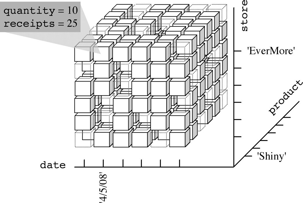
The concept of dimension gave life to the broadly used metaphor of cubes to represent multidimensional data. According to this metaphor, events are associated with cube cells and cube edges stand for analysis dimensions. If more than three dimensions exist, the cube is called a hypercube. Each cube cell is given a value for each measure. Figure 1-10 shows an intuitive representation of a cube in which the fact is a sale in a store chain. Its analysis dimensions are store, product and date. An event stands for a specific item sold in a specific store on a specific date, and it is described by two measures: the quantity sold and the receipts. This figure highlights that the cube is sparse—this means that many events did not actually take place. Of course, you cannot sell every item every day in every store.
Figure 1-10:The three-dimensional cube modeling sales in a store chain: 10 packs of Shiny were sold on 4/5/2008 in the EverMore store, totaling $25.
|
||||
If you want to use the relational model to represent this cube, you could use the following relational schema:
SALES (store, product, date, quantity, receipts)
Here, the underlined attributes make up the primary key and events are associated with tuples, such as <'EverMore', 'Shiny', '04/05/08', 10, 25>. The constraint expressed by this primary key specifies that two events cannot be associated with an individual store, product, and date value combination, and that every value combination functionally determines a unique value for quantity and a unique value for receipts. This means that the following functional dependency holds:
To avoid any misunderstanding of the term event, you should realize that the group of dimensions selected for a fact representation singles out a unique event in the multidimensional model, but the group does not necessarily single out a unique event in the application domain. To make this statement clearer, consider once again the sales example. In the application domain, one single sales event is supposed to be a customer's purchase of a set of products from a store on a specific date. In practice, this corresponds to a sales receipt. From the viewpoint of the multidimensional model, if the sales fact has the product, store, and date dimensions, an event will be the daily total amount of an item sold in a store. It is clear that the difference between both interpretations depends on sales receipts that generally include various items, and on individual items that are generally sold many times every day in a store. In the following sections, we use the terms event and fact to make reference to the granularity taken by events and facts in the multidimensional model.
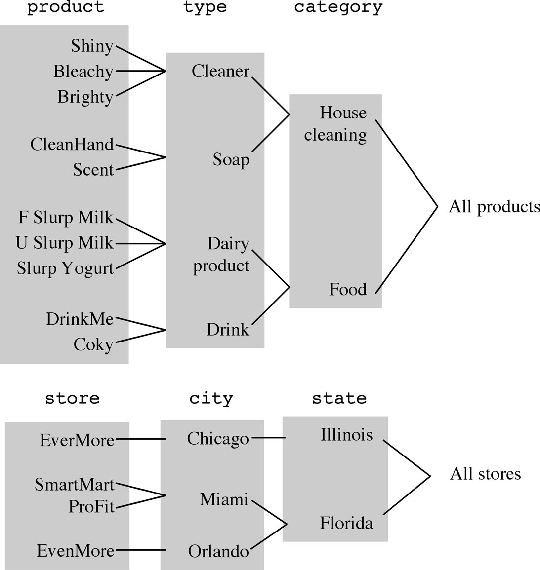
Normally, each dimension is associated with a hierarchy of aggregation levels, often called roll-up hierarchy. Roll-up hierarchies group aggregation level values in different ways. Hierarchies consist of levels called dimensional attributes. Figure 1-11 shows a simple example of hierarchies built on the product and store dimensions: products are classified into types, and are then further classified into categories. Stores are located in cities belonging to states. On top of each hierarchy is a fake level that includes all the dimension-related values. From the viewpoint of relational theory, you can use a set of functional dependencies between dimensional attributes to express a hierarchy:
store → city → state
In summary, a multidimensional cube hinges on a fact relevant to decision-making. It shows a set of events for which numeric measures provide a quantitative description. Each cube axis shows a possible analysis dimension. Each dimension can be analyzed at different detail levels specified by hierarchically structured attributes.
The scientific literature shows many formal expressions of the multidimensional model, which can be more or less complex and comprehensive. We'll briefly mention alternative terms used for the multidimensional model in the scientific literature and in commercial tools.
Figure 1-11: Aggregation hierarchies built on the product and store dimensions
The fact and cube terms are often interchangeably used. Essentially, everyone agrees on the use of the term dimensions to specify the coordinates that classify and identify fact occurrences. However, entire hierarchies are sometimes called dimensions. For example, the term time dimension can be used for the entire hierarchy built on the date attribute. Measures are sometimes called variables, metrics, properties, attributes, or indicators. In some models, dimensional attributes of hierarchies are called levels or parameters.
Note:The fact and cube terms are often interchangeably used. Essentially, everyone agrees on the use of the term dimensions to specify the coordinates that classify and identify fact occurrences. However, entire hierarchies are sometimes called dimensions. For example, the term time dimension can be used for the entire hierarchy built on the date attribute. Measures are sometimes called variables, metrics, properties, attributes, or indicators. In some models, dimensional attributes of hierarchies are called levels or parameters.
The information in a multidimensional cube is very difficult for users to manage because of its quantity, even if it is a concise version of the information stored to operational databases. If, for example, a store chain includes 50 stores selling 1000 items, and a specific data warehouse covers three-year-long transactions (approximately 1000 days), the number of potential events totals 50 × 1000 × 1000 = 5 × 10(7th). Assuming that each store can sell only 10 percent of all the available items per day, the number of events totals 5 × 10(6th). This is still too much data to be analyzed by users without relying on automatic tools.
You have essentially two ways to reduce the quantity of data and obtain useful information: restriction and aggregation. The cube metaphor offers an easy-to-use and intuitive way to understand both of these methods, as we will discuss in the following paragraphs.
1.5.1 Restriction
Restricting data means separating part of the data from a cube to mark out an analysis field. In relational algebra terminology, this is called making selections and/or projections.
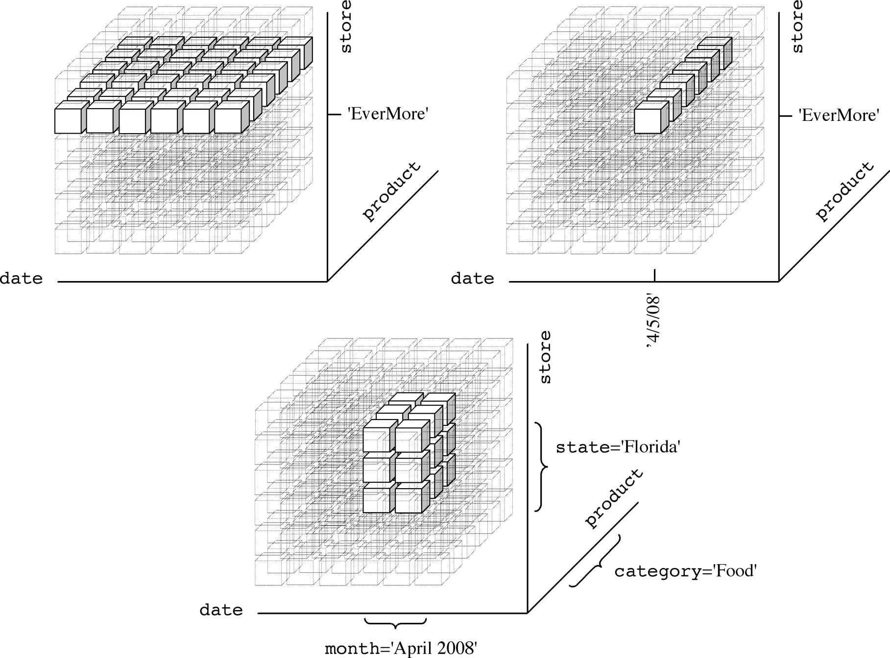
The simplest type of selection is data slicing, shown in Figure 1-12. When you slice data, you decrease cube dimensionality by setting one or more dimensions to a specific value. For example, if you set one of the sales cube dimensions to a value, such as store='EverMore', this results in the set of events associated with the items sold in the EverMore store. According to the cube metaphor, this is simply a plane of cells—that is, a data slice that can be easily displayed in spreadsheets. In the store chain example given earlier, approximately 10(5th) events still appear in your result. If you set two dimensions to a value, such as store='EverMore' and date='4/5/2008', this will result in all the different items sold in the EverMore store on April 5 (approximately 100 events). Graphically speaking, this information is stored at the intersection of two perpendicular planes resulting in a line. If you set all the dimensions to a particular value, you will define just one event that corresponds to a point in the three-dimensional space of sales.
Dicing is a generalization of slicing. It poses some constraints on dimensional attributes to scale down the size of a cube. For example, you can select only the daily sales of the food items in April 2008 in Florida (Figure 1-12). In this way, if five stores are located in Florida and 50 food products are sold, the number of events to examine changes to 5 × 50 × 30 = 7500.
Finally, a projection can be referred to as a choice to keep just one subgroup of measures for every event and reject other measures.
Figure 1-12: Slicing and dicing a three-dimensional cube
1.5.2 Aggregation
Aggregation plays a fundamental role in multidimensional databases. Assume, for example, that you want to analyze the items sold monthly for a three year period. According to the cube metaphor, this means that you need to sort all the cells related to the days of each month by product and store, and then merge them into one single macrocell. In the aggregate cube obtained in this way, the total number of events (that is, the number of macrocells) is 50 × 1000 × 36. This is because the granularity of the time dimensions does not depend on days any longer, but now depends on months, and 36 is the number of months in three years. Every aggregate event will then sum up the data available in the events it aggregates. In this example, the total amount of items sold per month and the total receipts are calculated by summing every single value of their measures (Figure 1-13). If you further aggregate along time, you can achieve just three events for every store-product combination: one for every year. When you completely aggregate along the time dimension, each store-product combination corresponds to one single event, which shows the total amount of items sold in a store over three years and the total amount of receipts.
Figure 1-13: Time hierarchy aggregation of the quantity of items sold per product in three stores. A dash shows that an event did not occur because no item was sold.
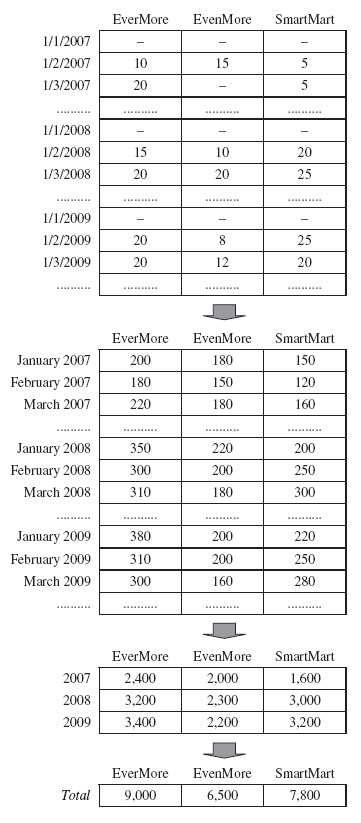
Figure 1-14: Two cube aggregation levels. Every macro-event measure value is a sum of its component event values.
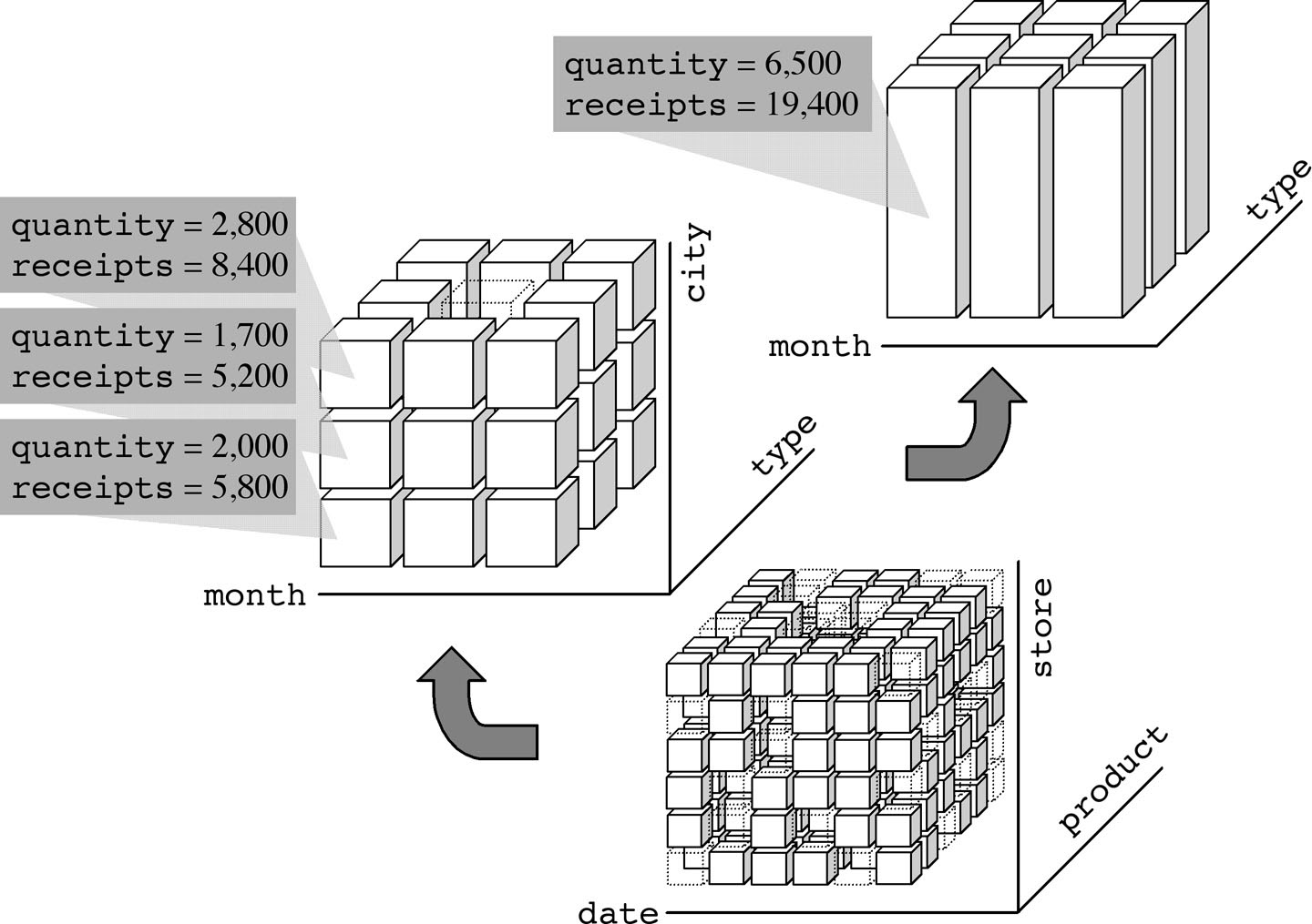
You can aggregate along various dimensions at the same time. For example, Figure 1-14 shows that you can group sales by month, product type, and store city, and by month and product type. Moreover, selections and aggregations can be combined to carry out an analysis process targeted exactly to users' needs.
1.6 Meta-data
The term meta-data can be applied to the data used to define other data. In the scope of data warehousing, meta-data plays an essential role because it specifies source, values, usage, and features of data warehouse data and defines how data can be changed and processed at every architecture layer. Figures 1-3 and 1-4 show that the meta-data repository is closely connected to the data warehouse. Applications use it intensively to carry out data-staging and analysis tasks.
According to Kelly's approach, you can classify meta-data into two partially overlapping categories. This classification is based on the ways system administrators and end users exploit meta-data. System administrators are interested in internal meta-data because it defines data sources, transformation processes, population policies, logical and physical schemata, constraints, and user profiles. External meta-data is relevant to end users. For example, it is about definitions, quality standards, units of measure, relevant aggregations.
Meta-data is stored in a meta-data repository which all the other architecture components can access. According to Kelly, a tool for meta-data management should
- allow administrators to perform system administration operations, and in particular manage security;
- allow end users to navigate and query meta-data;
- use a GUI;
- allow end users to extend meta-data;
- allow meta-data to be imported/exported into/from other standard tools and formats.
As far as representation formats are concerned, Object Management Group (OMG, 2000) released a standard called Common Warehouse Metamodel (CWM) that relies on three famous standards: Unified Modeling Language (UML), eXtensible Markup Language (XML), and XML Metadata Interchange (XMI). Partners, such as IBM, Unisys, NCR, and Oracle, in a common effort, created the new standard format that specifies how meta-data can be exchanged among the technologies related to data warehouses, business intelligence, knowledge management, and web portals.
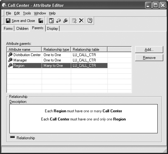
Figure 1-15 shows an example of a dialog box displaying external meta-data related to hierarchies in MicroStrategy Desktop of the MicroStrategy 8 tool suite. In particular, this dialog box displays the Calling Center attribute parent attributes. Specifically, it states that a calling center refers to a distribution center, belongs to a region, and is managed by a manager.
Figure 1-15: Accessing hierarchy meta-data in MicroStrategy
Note See Barquin and Edelstein, 1996; Jarke et al., 2000; Jennings, 2004; and Tozer, 1999, for a comprehensive discussion on meta-data representation and management.
More on data warehouse design:
- Continue to the next section: Best practices for data warehouse access and reports
- Download a free PDF of this chapter: "An Introduction to Data Warehousing"
- To purchase the book or similar titles, visit McGraw-Hill
- Read other excerpts from data management books in the Chapter Download Library.